Catenary Calculator (Forces & Co-ordinates)
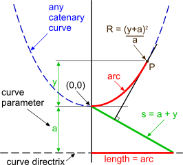
Fig 1. Theoretical Catenary diagram
Theoretical Catenary
A catenary is a theoretical curve with the x,y relationship: y = a.[cosh(x/a) – 1] (Fig 1). Where 'a' is the curve's parameter (a = Fx / w) and defines the shape of the catenary: i.e. a flat catenary has a large parameter and a tall catenary has a small parameter. Some of the other relationships between the parameter and the curve are shown in Fig 1 (R is the radius of the curve at point P).
Practical Catenary
Whilst this curve is a theoretical mathematical shape, it is also something that occurs naturally every time you hang a cord of zero bending stiffness and infinite axial stiffness between any two points (co-ordinates).
CalQlata is concerned only with the practical use of this configuration and has therefore tailored this calculator around finding relative co-ordinates, forces & angles at both ends and at any point along its length (Fig 2).
Whilst a true catenary curve will occur naturally in a cable with zero bending stiffness (e.g. chain or string), the theory may equally be applied with reasonable accuracy to a cable with inherent bending stiffness if sufficiently long.
Refer to Tight Catenary below for a definition of the configuration of electricity or anchor cables.
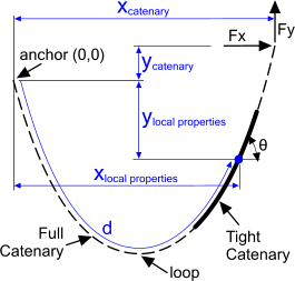
Fig 2. Practical Catenary diagram
Definition of a Catenary
The two practical properties defining a natural catenary are:
1) the horizontal force (Fx) in the cable is constant throughout its length, and;
2) the vertical force (Fy) in the cable at any point is equal to the weight of cable that point is carrying (i.e. Fy = 0 at the bottom of the loop).
The angle of the cable at any point is determined by resolving these forces, e.g. TAN⁻¹(Fy/Fx)
'Tight' Catenary
CalQlata defines a tight catenary (see Fig 2) as one with no loop (i.e. there is no point in its length where Fy=0) the shape of which is less affected by inherent stiffness.
The shape of any tight catenary can be exactly superimposed on a full catenary with the same horizontal force (Fx). Its position within this catenary is defined by the vertical loads (Fy) at each end, which will be identical to the loads in the full catenary at those end points.
Calculation options 'Catenary (x,y)' and 'Catenary (Fx,Fy)' both produce a 50-point co-ordinate listing of the curve generated in the Catenary calculator that you can copy and paste into your preferred spreadsheet program (e.g. Microsoft Excel).
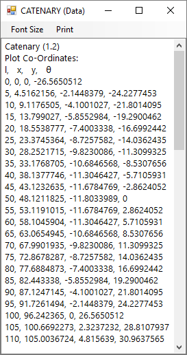
Fig 3. Co-Ordinate Listing
Catenary Calculator - Technical Help
Units
You may use any units you like, but you must be consistent.
Calculations
As Catenary is a calculator designed for practical use its '0,0' co-ordinates are set at one end of the cord (Fig 2 defined in the calculator as the anchor) and not at its theoretical origin (Fig 1). You simply pick up the other end and position it relative to the anchor by adjusting the x,y co-ordinates of the free end or by varying vertical (Fy) and horizontal (Fx) forces. Catenary calculates the end conditions along with its local properties at your designated distance ('d') from its anchor.
You enter:
The length and weight per unit length of the cable along with either its free-end position ('Option: x,y') or its lift/pull forces ('Option: Fx,Fy') and Catenary will calculate either the forces or the position of the free-end, along with the in-line forces and angles at both ends.
You can also enter a distance ('d') from the 'Anchor end of the catenary and Catenary will calculate the same information at this position as that provided at each end.
Plotting your Curve
In addition to the calculator's graphical presentation of the curve, calculation options: 'x,y' and 'Fx,Fy' both produce a 50-point co-ordinate listing of the curve generated in the Catenary calculator that you can copy and paste into your preferred spreadsheet program (e.g. Microsoft Excel).
The co-ordinate listing is generated at the bottom of the Data Listing page of the calculator, headed by 's' (distance along curve from origin), x (horizontal distance to 's'), y (vertical distance to 's'), θ (angular orientation of curve @ 's'). Each co-ordinate is separated by a comma (Fig 3).
To generate a plot of your curve, simply:
1) select and copy the full list of co-ordinates (with or without the 's, x, y, θ' heading - your choice) and paste it into your spreadsheet
2) Unless your spreadsheet automatically converts Text to Columns, you will need to do this yourself the first time you paste data into your spreadsheet
a) Menu item: 'Data'>'Text to Columns'
b) Select 'Delimited'
c) Click 'Next' button
d) Deselect 'Tab' and select 'Comma'
e) Click 'Finish' button
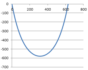
Fig 4. Typical Catenary Curve
3) You then select the two centre columns of data (with or without the 's, x, y, θ' heading - your choice) and insert a chart
a) Menu item: 'Insert>Chart>Scatter'
b) Select 'Scatter with smooth lines'
4) Adjust axes (chart window size) so that the grid scales are equal (Fig 4)
5) You can then copy and paste new co-ordinate listings over the current list as many times as you wish. The text will be automatically converted to columns and the plot will be automatically updated every time you over-paste a new set of co-ordinates
Please Note: All our calculators use full-stops (.) for the decimal point and commas (,) for the thousand separator. If your computer reverses this arrangement, you will need to swap them using Microsoft's 'Word' (or similar word precessor) before copying the output data into 'Excel' (or similar spreadsheets) for further processing.
Self-Check
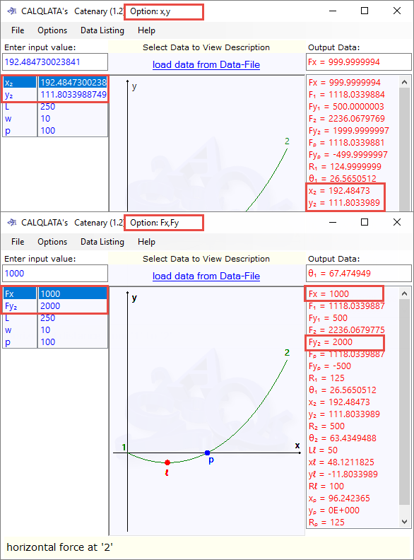
Because the two principal calculation options ('Fx,Fy' and 'x,y') use different formulas and procedures ('x,y' is iterative and 'Fx,Fy' is direct) a calculation performed using one method acts as a self-checking facility for the other.
Apart from carrying out your own hand calculations to verify this calculator, the self-checking procedure may be accomplished as follows:
Enter your input variables in either calculation option 'Fx,Fy' or 'x,y', activate the 'Data Listing' window and simply swap between the calculation options.
Accuracy
The 'Fx,Fy' option is the most accurate and consistent and should be used for exact results. You could, however, perform the 'x,y' calculation then switch to the 'Fx,Fy' option entering specific (rounded off) values for free end forces to achieve an exact result (Fig 5).
Whilst this is considered by CalQlata to be unnecessary (the 'x,y' option iterates to within
±1.0E-08) caution should be given to the fact that even though the error margin for the iterative x,y calculation option is small, repeated swapping from one to the other with the same input values will compound the error. It is advisable therefore, either to swap between the calculation option no more than 5 or 6 times or to use the output from a Fx,Fy calculation.
Further Reading
You will find further reading on this subject in reference publications(3 & 9)

